
Tutorial
Things to prepare before using SimRNAweb
It is best to gather as much information as possible before using SimRNAweb to do a simulation. SimRNAweb can do de novo folding and can often solve a short hairpin sequence quite successfully. However, most of the interesting RNA structures are complex. Secondary structure information alone may not be adequate to ensure that a correct prediction is obtained. Therefore, it may be necessary to obtain information on tertiary structure.
- [REQUIRED] an RNA sequence or a PDB/mmCIF format RNA structure (remember to select appropriate input type for your input structure).
- [REQUIRED] If you are using a PDB/mmCIF format input structure, please ensure that your data is clean. Verify that all 5 atoms of SimRNA (P, C4', N1/N9, C2, C4/C6) are present, and there is no duplication of residues.
- [Facultative] secondary structure (base pairing information) of the RNA, if available. This can come from either an experimental source (better) or a calculated result from a secondary structure prediction program (less reliable). Note: please read the explanation below for information on how to express pseudoknots with the dot bracket notation.
- [Facultative] any tertiary structure information (long range distance interactions), if available.
- [(For advanced users) REQUIRED] If the input PDB file contains labels for modified bases, these locations must be found in the PDB file and modified such that the residue name is read as one of the standard bases (A, C, G or U). This means that the HETATM tag must be changed to ATOM when this is the case. In general, this action should be sufficient as long as the modified residues have the following essential atoms: C4', P, N1, C2 and C4 (for pyrimidines) or C4', P, N9, C2, C6 (for purines). If any of these atoms are missing, then it is probably better to delete the modified residue altogether and submit the structure with the complete sequence; i.e, the sequence must contain the missing residue(s).
Example input
In Figures 1a-g, we show various examples of using restraints with sequences and PDB files under various circumstances for PDB id 1L2X.
|
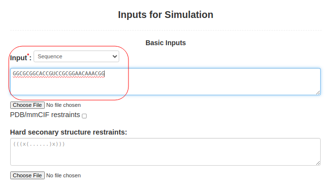
(1. Sequence alone) When only the sequence is submitted to SimRNAweb, the RNA sequence should be pasted into Box (3): Input: **select "Sequence" as input typeGGCGCGGCACCGUCCGCGGAACAAACGG |
Figure 1a. Submitting sequence alone to SimRNAweb. |
|
(2. Sequence and secondary structure) When the sequence is submitted along with the structure of a pseudoknot (perhaps obtained from RFAM or from SHAPE data), Boxes (3) and (4) are used. The sequence above is submitted in Box (3), as above GGCGCGGCACCGUCCGCGGAACAAACGGand the pseudoknot structure is introduced by submitting two lines of secondary structure corresponding to the two overlapping helices in the secondary structure field (Box (4)), ..(((((......))))).......... .........(((.............))) You can use either Hard secondary structure restraints or Soft secondary structure restraints (advanced option), or even both of them with different secondary structures. The hard secondary structure restraints force SimRNA to create the specified secondary structure, while the soft restraints wait for SimRNA to detect the base pair during simulation. With a bonus, they assist in maintaining the base pair once detected.
Note that pseudoknot restraints are expressed by including an
additional line with the entangled helix on a second line. This can
be done up to as many lines as needed to specify any very deeply
entangled pseudoknots. This notation allows clear specification for
more than one pseudoknot, as opposed to the usual notation
|
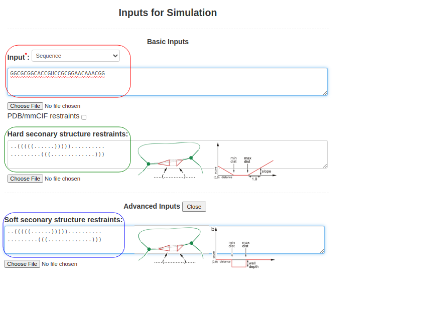
Figure 1b. Submitting sequence along with secondary structure restraints to SimRNAweb. |
|
(3. Refining a 3D structure) When starting with a structure in PDB/mmCIF Format (e.g., 1l2x_rna_clust0.pdb), one should select the PDB/mmCIF in the Box(3) upload either format in Box (4) of the submission form. In principle, the secondary structure restraints listed in Box (5) or (6) are not absolutely required. However, in general, unless one wishes to continue (or restart) a simulation from some intermediate point without restraints, there is little reason to submit a correct PDB structure and do a simulation on it. Maybe there is a situation where this might be necessary, but in general, the purpose would (probably) be refinement. The secondary structure information is entered in Box (5) or (6) as before, ..(((((......))))).......... .........(((.............))) and the input PDB structure file: 1l2x_rna_clust0.pdb is entered in Box (3). |
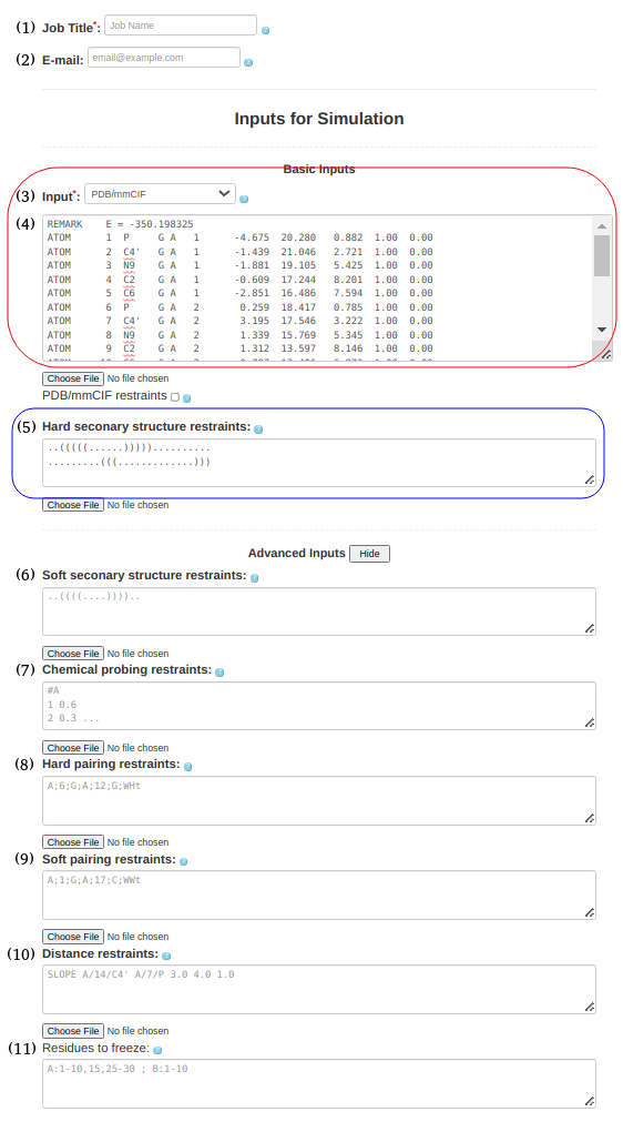
Figure 1c. Submitting a PDB file along with secondary structure restraints to SimRNAweb. |
|
(4. Refining a 3D structure with freezing residues, distance restraints, and hard secondary structure restraints) It is also possible to submit a PDB/mmcif format (Box (4)) with hard secondary structure restraints (Box (5)), ..(((((......))))).......... .........(((.............))) include the PDB structure file (1l2x_rna_clust0.pdb) for refinement in Box (11), specify frozen residues in the PDB file in Box (6), A:3-7, 14-18 and upload any additional distance restraints into Box (10) using a text file with the appropriate syntax (e.g., 1l2x_restraints.txt) SLOPE A/14/C4' A/7/P 3.0 4.0 1.0 WELL A/14/C4' A/7/P 4.0 6.0 1.0 NOTE: Please see the last Section of this help document to find more information on formatting and combining distance restraints (including some applied examples). |
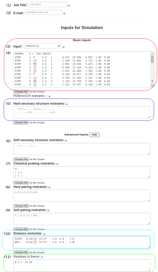
Figure 1d. Submitting a PDB file to SimRNAweb along with secondary structure restraints, distance restraints, and frozen parts of the structure (based on the PDB file). |
|
(5. Sequence with pairing restraints) It is possible to provide information about the secondary structure in the pairing format. As before, the input type in Box (3) must be selected as "Sequence," and the sequence must be uploaded in box (4). GGCGCGGCACCGUCCGCGGAACAAACGGSimilarly to hard and soft secondary structure restraints, you can utilize hard or soft pairing restraints by pasting the pairing information in Box (8) or (9). A;3;C;A;18;G;WWc A;4;G;A;C;17;WWc A;5;C;A;G;16;WWc A;6;G;A;C;15;WWc A;7;G;A;C;14;WWc A;10;G;A;28;C;WWc A;11;C;A;27;G;WWc A;12;C;A;26;G;WWc The current input format for constraints on non-canonical base pairs requires the user to specify the base pair type. This feature is particularly useful for known motifs based on non-canonical interactions, such as k-turns, e-loops and others. The example already included in the paper is the G-quadruplex, which is based solely on non-canonical base pairs, and where the specific interactions are known (the user can assume which residue pairs with which residue and what type of base pair is formed). We recognize that predicting the specific nature of non-canonical base pairs is difficult outside of the usual motifs. Most methods that can predict non-canonical pairs only do so at the residue pair level, but they rarely specify a concrete type of non-canonical base pair. If the user is unsure of the base pair type, the new soft constraints feature allows multiple alternative base pairing possibilities to be specified for the same pair of residues, allowing for an ambiguous definition of base pairs.
|
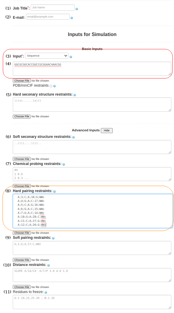
Figure 1e. submitting a sequence to SimRNAweb along with secondary structure restraints and distance restraints. |
(6. Sequence with soft secondary structure restraints and chemical restraints) As before input type (Box (3)) must be "Sequence" and be entered in the Box (4)
GCUUCAUAUAAUCCUAAUGAUAUGGUUUGGGAGUUUCUACCAAGAGCCUUAAACUCUUGAUUAUGAAGUGSecondary structure should be pasted in Box (6)
((((((((...((((((.........))))))........((((((.......))))))..)))))))).chemical probing information should be provided in Box (7)
#A
1 0.0
2 0.0
3 0.0
4 0.0
5 0.12
6 0.06
7 0.02
8 0.4
11 0.28
12 0.03
13 0.0
14 0.0
15 0.0
16 0.02
17 0.06
18 0.2
19 0.25
20 0.17
21 0.05
22 0.48
23 0.21
...
the full input for chemical probing can be found here (just add #A at the begining of the chemical probing data)
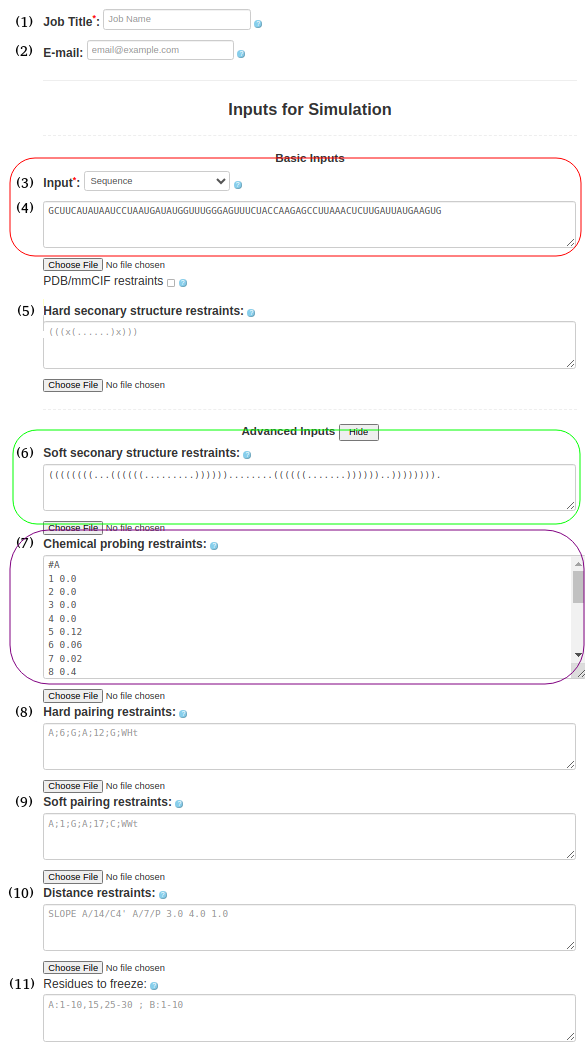
Figure 1f. submitting a sequence to SimRNAweb along with secondary structure restraints and distance restraints.
NOTE: Regarding the interpretation of chemical probing data, SimRNAWeb v2.0 employs a simplistic approach focused solely on base pairing, while the reactivity to chemical probes can be influenced by factors beyond the status of base pairing. Thus, on one hand, this method does not accommodate the inherent noise in chemical probing data, and on the other, it does not endeavor to interpret complex 3D structural features that may affect actual reactivity. Nonetheless, these types of restraints serve merely as a bias and do not drive the simulation to completely fulfill and potentially overfit the restraints. The current implementation enables users to input data that guide the simulation towards conformations enriched in regions of low reactivity in chemical probing experiments, which are preferably (but not exclusively) involved in forming helices or long-range interactions
Detailed description of inputs
1. Format of sequence input files
The input data is written in a single line in a basic text file with the sequence of RNA (both upper and lower cases are acceptable). For example:
AGACUGCUGAGAGACC
There should be nothing but the desired sequence or sequences contained in the file because the program will read everything in the file as though it were part of a sequence. There should be no additional spaces either.
To have more than one RNA chain as an input, the user must separate the different chains by white spaces. For example:
AAGCUA AAAGCUGGGCU
2. Format of secondary structure restraint files
If the user wants to provide secondary structure restraints, the contents of the restraint file should be in the following one-line format:
.((((......)))).
Or, when pseudoknots are involved, several lines can be provided depending on the characteristics of the pseudoknot. For example, if there is only one pseudoknot, then the following is sufficient:
.((((......)))).
......(........)
If more than one pseudoknot is involved, each one should be written on a separate line. For example, the following structure would involve two pseudoknots:
((((.......))))...............((((.........))))).
......((((.............))))......................
..................((((..............)))).........
Comments:
- In general, it is good policy to write the dominant secondary structure on the first line and place only single hairpin loops closing the pseudoknots on subsequent lines; however, this is not strictly required.
-
The program reads in the constraints line by line. Therefore, the
following input
(((......)))
can also be written as follows(..........) .(........). ..(......)..
It is important to emphasize that the data for secondary structure and pseudoknots must be listed on subsequent lines regardless of how the data is specified. Otherwise, SimRNA will assume that there is a second chain, and it is likely that an error will occur. -
Constraints can also be applied to multichain problems. For example, in the case of two chains, restraints can be written as follows:
AAAACCCCUUUU AAAACCCCUUUU
((((....(((( ))))....))))
The above example will form a double-stranded RNA (dsRNA) stem with an interior loop containing poly(C). When the sequence is written as above in the restraint file, the first line is ignored.
-
If more than two chains are involved, this can also be accommodated by the above scheme. For example, constraints on four chains could be written as follows
AAAACCCCUUUU AAAACCCCUUUU AAAAGGGGAAAA AAAAGGGGAAAA
((((....(((( ))))....)))) ............ ............
............ ....((((.... ....)))).... ............
....((((.... ............ ............ ....))))....
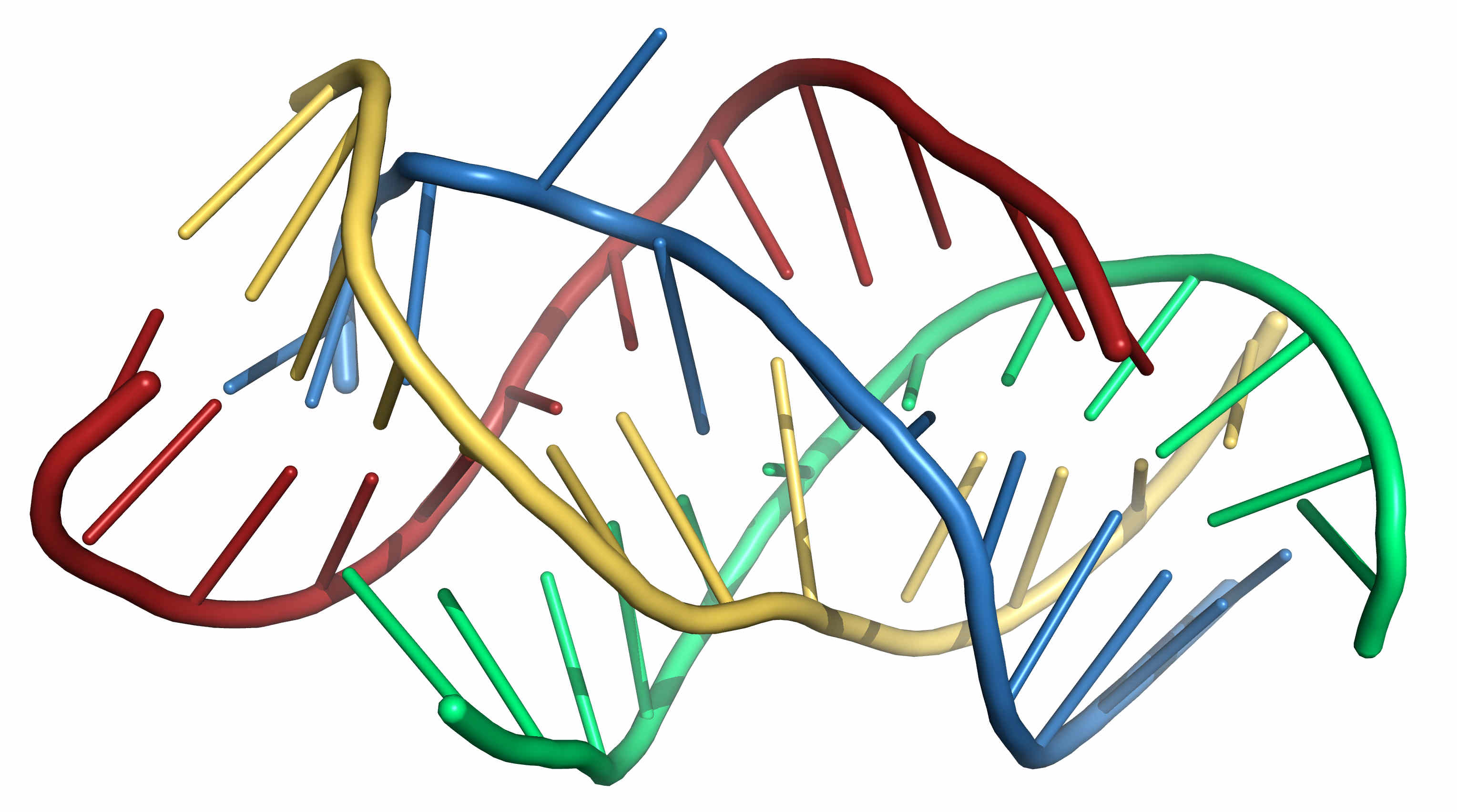
Figure 3. A possible 3D structure of the four sequence shown above folded under the proposed restraints using SimRNA. -
In general, there is a variety of ways that this file can be written. However, clarity is probably the most important thing to remember.
-
Finally, please note that SimRNAweb doesn’t allow the user to exclude the possibility of base pairing using the secondary structure constraints file. Thus, even the dot “.” does not prohibit the formation of base pairing.
3. Format of structure input files
The user requests starting the calculation with a structure provided by the user in PDB format.
Essentially, a PDB file is cleaned (water, ions, non-standard residues are removed) with `rna-pdb-tools` to get a file "SimRNA ready". However, these tools simply follow orders (all muscle and no brain). Therefore, it is wise when the user prepares the PDB files to avoid any inadvertent misinterpretation of desired structural information on the part of the automated tools.
Hence, although a fair amount of flexibility is built into SimRNAweb, there are some important caveats to keep in mind.
- SimRNAweb can read the HETATM tags. Therefore, most of the time, it is sufficient to simply change a modified residue name to its unmodified name (A, C, G or U) without any additional effort on editing the PDB file. However, the user should make sure that the HETATM references point to desired parts of the RNA structure: not ligands or other molecules that may have been needed to crystallize the RNA structure in a particular state or are part of the crystal structure that was obtained. The outcome of a job submission for such uninspected PDB files simply cannot be predicted. Therefore, it is the user's responsibility to be sure that SimRNAweb is being fed the intended RNA structure and not garbage.
- Sometimes, some of the backbone atoms are present for a residue, but important parts (or all) of the base are missing. Also, sometimes, to crystallize the structure, very special residues are constructed that do not have the same essential atoms needed by SimRNA. The essential atoms are C4′,P,N1,C2,C4 (for any pyrimidine residues) or C4′,P,N9,C2,C6 (for any purine residues). If any of these critical atoms are missing, then all of the atoms of the residue (including the backbone) should be removed from the PDB file, and the correct sequence (including the missing base) should be inserted in Box (3), as in the examples shown above. Therefore, it is important to examine the PDB file for missing or incomplete information. If any part of this information is missing, the structure is inadequately defined and will be rejected by SimRNAweb.
- Another problem is modified bases. In some cases, simply changing HETATM to ATOM and changing the residue name to the unmodified base (A, C, G or U) is sufficient. However, if the modification changes the name of any one of the essential atoms that are used by SimRNA, this will be the same as having an incompletely defined residue. After changing the tag and the name of the residue, the residue atoms should be inspected to verify that the critical atoms C4′,P,N1,C2,C4 (for a pyrimidine) or C4′,P,N9,C2,C6 (for a purine) are present. If any of these are missing, the residue should be removed from the PDB file and only specified in the sequence (submitted in Box (3), as explained above).
- SimRNAweb will insert the 5′ most phospate if it is missing. However, it does not hurt to verify whether it is present or not, because the way of doing this insertion presently is to rename the O5' atom to a P atom at the 5′-most position. In general, this should not introduce any issues, particularly when SimRNA is converted from its reduced representation to the all atom representation after a brief simulation. Nevertheless, it should be kept in mind that this amounts to a "quick fix" and may not be what the user genuinely wants. If so, then the user will need to find a way to insert the desired 5′ P in a more amenable position.
4. Distance restraint command formats
In SimRNA, distance restraints can be defined for any pair of atoms used in SimRNA representation, as well as to the central point of the nucleic acid base: for pyrimidines P, C4′, N (N1, N9), C2, C4 and for purines P, C4′, N9, C2, C4 and C6 (for purines) and the the middle of the base (label MB).
The restraints come in two basic forms: WELL
and SLOPE. A typical WELL restraint
effectively "captures" the two beads when they come within a
prescribed distance from each other as in Figure 4a, where the
penalty is zero when the distance between the orange and red bead is
outside of the well, and some negative number when inside the
well. This means nothing happens until it finds the hole. A
typical SLOPE restraint penalizes any region outside
the zone where the penalty is zero as in Figure 4b.
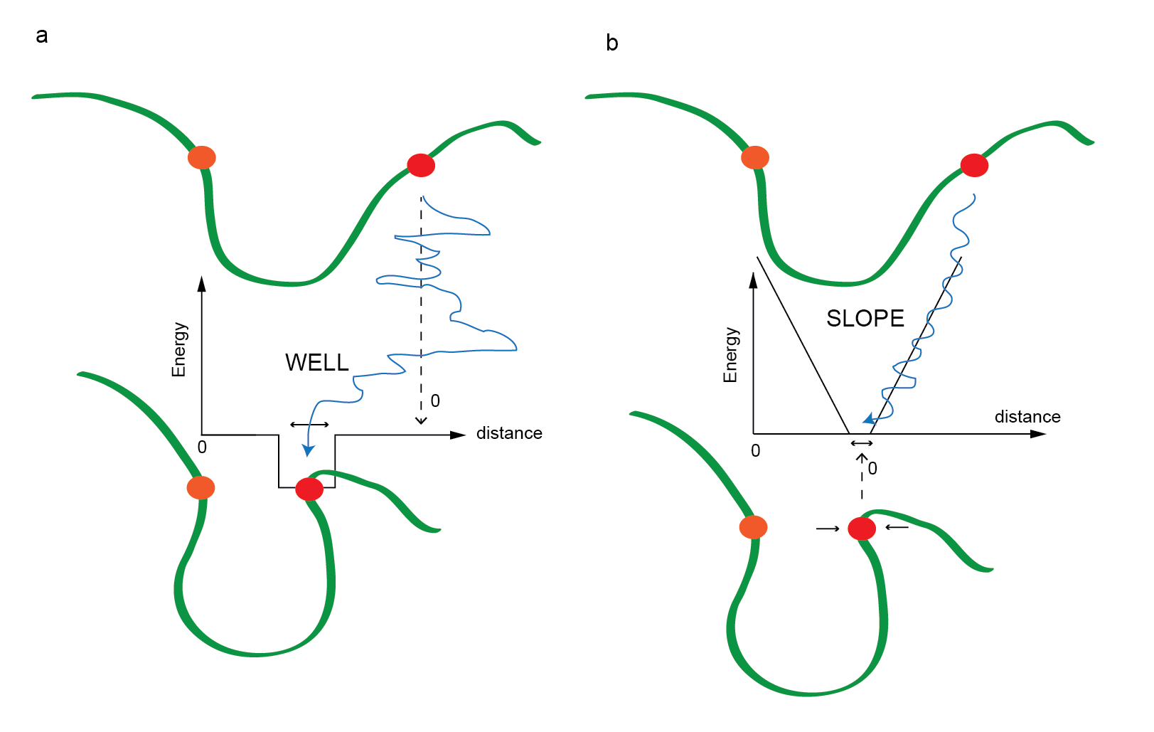
Figure 4. A cartoon describing the way restraints affect the
interaction between two beads: here orange is the reference bead and
the red bead is shown moving relative to the orange bead. a)
A WELL restraint where outside the hole, the red bead
moves freely and inside the hole, it is trapped to a specific range.
b) A SLOPE restraint where the penalty is zero when the
distance between the beads is inside the zone, and outside this, the
beads are either pulled together or pushed away.
The restraints come in two basic forms: WELL
and SLOPE. A typical WELL restraint
effectively "captures" the two beads when they come within a
prescribed distance from each other as in Figure 4a, where the
penalty is zero when the distance between the orange and red bead is
outside of the well, and some negative number when inside the
well. This means nothing happens until it finds the hole. A
typical SLOPE restraint penalizes any region outside
the zone where the penalty is zero as in Figure 4b.
Figure 4. A cartoon describing the way restraints affect the
interaction between two beads: here orange is the reference bead and
the red bead is shown moving relative to the orange bead. a)
A WELL restraint where outside the hole, the red bead
moves freely and inside the hole, it is trapped to a specific range.
b) A SLOPE restraint where the penalty is zero when the
distance between the beads is inside the zone, and outside this, the
beads are either pulled together or pushed away.
The WELL restraint is expressed by a single line in the restraints
file as follows:
WELL atom_1_id atom_2_id min_dist max_dist weight
The SLOPE restraint is expressed similarly as follows:
SLOPE atom_1_id atom_2_id min_dist max_dist weight
or (alternative for SLOPE):
DISTANCE atom_1_id atom_2_id min_dist max_dist weight
Example line in a restraints file:
SLOPE A/23/C4' C/45/P 5.5 8.5 1.0
WELL A/23/C4' C/45/P 6.5 7.5 1.0
where
A/23/C4' means atom C4' of nucleotide 23 in chain A
C/45/P means atom P in nucleotide 45 in chain C
5.5 [Å]: minimal distance where the weight is zero (for SLOPE)
6.5 [Å]: minimal distance where the weight is -1 (for WELL)
7.5 [Å]: maximal distance where the weight is -1 (for WELL)
8.5 [Å]: maximal distance where the weight is zero (for SLOPE)
1.0 weight of this restraint weight for both SLOPE
and WELL. For WELL, the value is -1
between 6.5 and 7.5 [Å], for SLOPE the value increases for distances
greater than 8.5 or less than 5.5 [Å].
This is an example of a multifunctional restraint that resembles Figure 5e.
Comments:
- If the input file is a PDB file, then the nucleotide numbers specified in the restraints file are according to numbering in input PDB file!
- In SimRNA representation, the atom name N represents the nitrogen that binds the base to the backbone. Hence,N corresponds to N1 for pyrimidines and N9 for purines! This label can also be used instead of N9 for purines and N1 for pyrimidines. SimRNA also permits the user to restrain the C2 atom or and also the C6 atom for purines or the C4 atom for pyrimidines.
- The user can also apply restraints for a middle atom of the base (pseudo atom) which is named MB! This is useful for restraining the bases such that they are only in contact but not specifically tied to some prescribed orientation such as Watson-Crick, or Hoogsteen edge, or whatever.
Restraint options
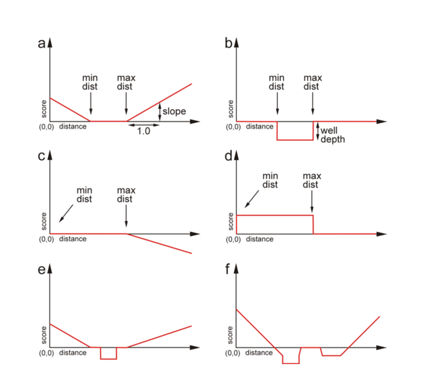
Figure 5. Examples of types of constraints. a) An elementary
function of type SLOPE that depends on the following
three parameters: the minimum distance, the maximum distance and the
slope. b) An elementary function of type WELL that
depends on three parameters: the minimum and maximum distance and
the depth of the well. c) A single SLOPE function with
negative weight. d) A single WELL function with
negative weight. e) A combination one SLOPE function
and one WELL function. f) A combination of
three SLOPE and two WELL functions, both
one WELL function and one SLOPE function
with negative weights.
A restraint can be thought of as a flexible tether that drives the selected atoms towards a certain distance by applying a penalty for distances that deviate from that range. It can also provide a reward when a desired distance is achieved. The penalty and reward are positive and negative contributions to the total energy of the simulated system, respectively.
There are two types of distance restraints: WELL
and SLOPE (the keyword DISTANCE can also
be used in the place of SLOPE). Both restraints
describe an inner zone between the specified minimum number and
maximum number (which can be the same
number). For SLOPE, the penalty within the inner zone
is zero, and all regions outside change linearly with distance by
the weight outside this zone. When the weight is positive,
the SLOPE forms a "V" shape or a "\_/" shape depending
on the size of the inner zone (Figure 5a). If the weight is
negative, the shape will be inverted, but the penalty in the inner
zone is always zero (for SLOPE). In the case
of WELL, a positive weight produces a divot "|_|" where
outside the zone, the value is zero and inside the well, the energy
is negative (Figure 5a). Changing the sign of the weight
for WELL means we create a wall or a stumbling block (a
positive penalty) in the inner zone.
The basic forms for SLOPE and WELL, where
the weight is positive, are shown in Figure 5a and b.
In the case of a SLOPE-type restraint, the two atoms
are tethered towards the region by applying a linear penalty that
corresponds to the degree of violation of the distance from the
desired region. When the distance between the atoms becomes equal to
the desired value, the value of the function reaches zero. The shape
of the function resembles a V, with a bottom that can
correspond to a single point or to a “flat” region (Figure
5a).
In case of a WELL-type restraint, the function is flat
and equals zero for any distance outside the desired range, while
the distances within the desired range correspond to the negative
value of the weight (Figure 5b).
Both the SLOPE and WELL restraint
functions can be “reversed” when a negative weight is applied
(c.f., Figures 5c and d). For example, applying
a SLOPE-type function with a negative weight can be
used as a repelling function (Figure 5c). This function can
be useful in simulations in which the user desires to study molecule
stretching between terminal residues, for example. On the other
hand, the WELL-type function can be applied with a
negative weight when the user wishes to define a distance range that
the atoms should avoid. When atoms are in the distance range
specified by WELL, an additional penalty is applied
(Figure 5d).
Any number of these two types of functions can be also combined in order to define complex restraints. The resulting function can adopt various shapes (Figures 5e and f). Therefore, the relative distance of two atoms under consideration can be described by a dedicated function or a linear combination of functions used as a part of the total scoring of the energy.
For both types of restraints, the user must specify the restraints in subsequent lines of the restraint file in the following format
ChX/i/atom_i ChY/j/atom_jmin_distmax_distweight
where examples are provided in the next
section. Here, ChX and ChY specify the
chain index (chain name can be the same or
different), i and j refer to the index of
the particular residue on the respective chain,
and atom_i and atom_j refer to the atom on
which the constraint is applied. Restraints of
type WELL are 0 except for the range
between min_dist and max_dist. For the
region between min/max
(min_dist↔max_dist), the value
becomes -1*weight.
Restraints of type SLOPE are 0 within the
range, min_dist↔max_dist. Outside
that range, a linear increasing positive penalty is added (the pair
of atoms are attracted to each other because there is less penalty
as they approach the region between min_dist
and max_dist). The value for the penalty is
dist_violation*weight.
Restraints for a given pair of atoms can be combined (added). It requires two (or more) lines to specify subsequent contributions.
For an applied example of using the above described restraints,
Figure 6 shows two examples where the secondary structure
restraints and distance restraints (WELL
and SLOPE) were used to improve the fit of the 3D
structure for two tRNA structures. The necessary restraint files and
sequence for folding 3L0U are also provided as an example on the
submission page of SimRNAweb, where the best structure using
this combination of restraints was 6.1 Angstroms RMSD (Figure
6a). Figure 6b provides the requisite files for PDB
structure 1EVV, where SimRNAweb produced one cluster with 6.5
Angstroms RMSD.
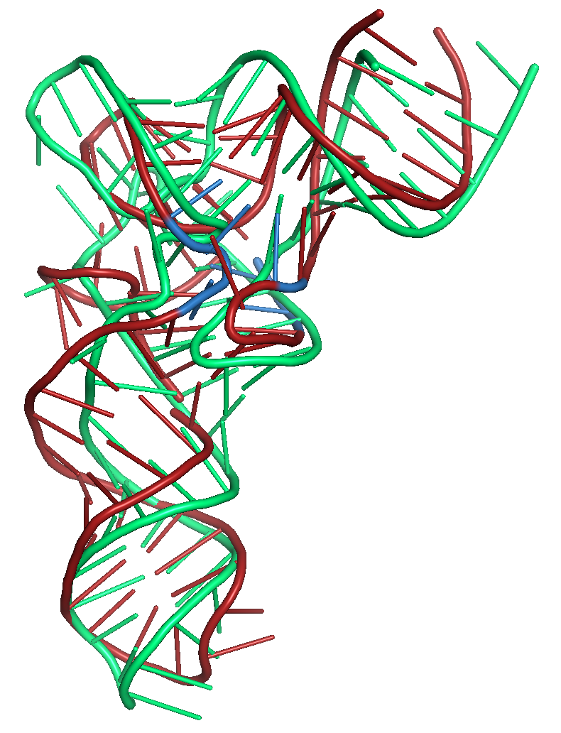
Figure 6a. Results of folding the sequence for PDB id 3L0U with secondary structure restraints and distance restraints using SLOPE and WELL. The
native structure is shown in green. The blue region shows
where the distance restraints were applied. The tRNA structure
has modified bases in this region of the structure.
|
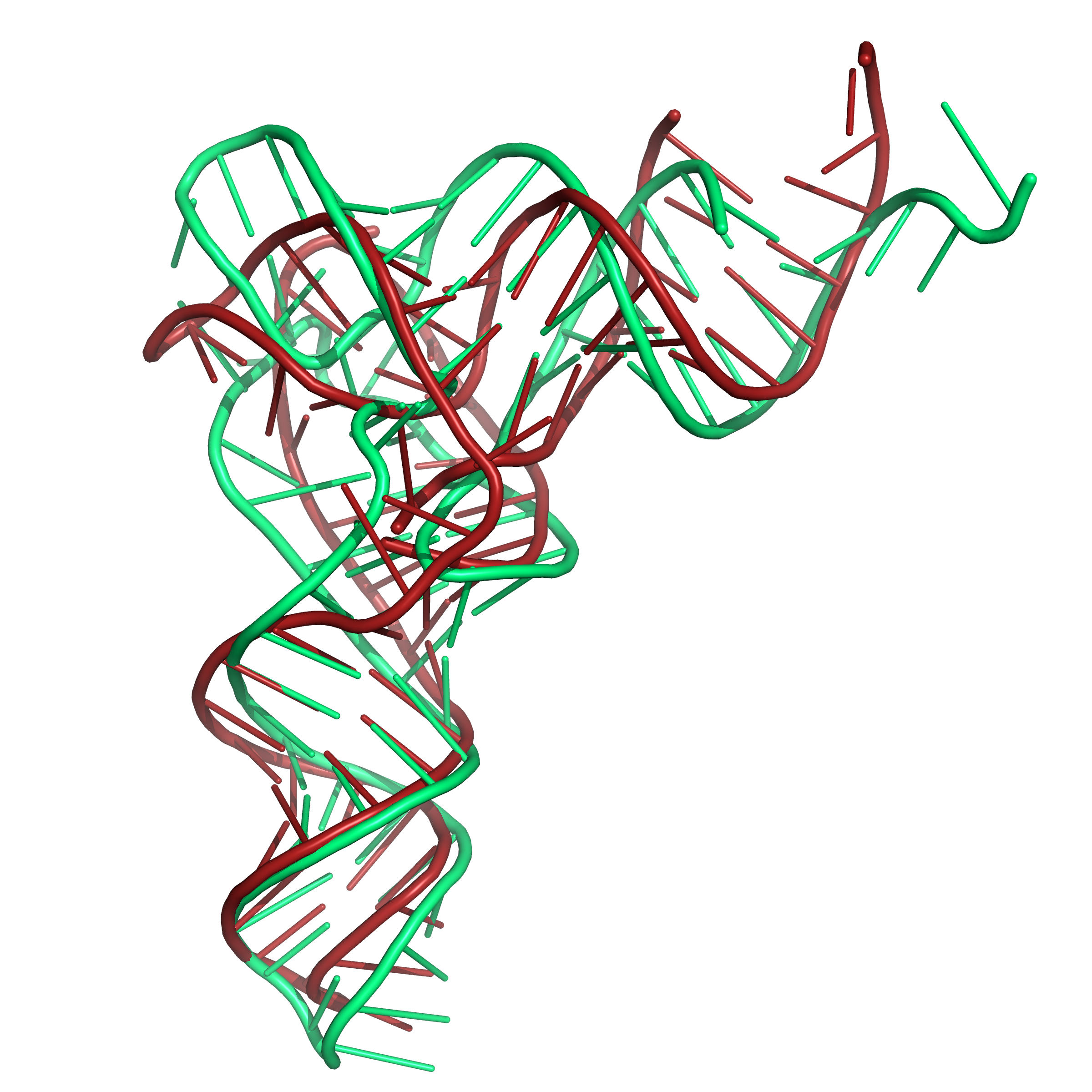
Figure 6b. Results of folding the sequence for PDB id 1EVV with secondary structure restraints and distance restraints using SLOPE and WELL. The
native structure is shown in green. Here also, the tRNA
structure has modified bases in this region of the structure.
|
5. Format of pairing restraint file
In SimRNA, pairing restraints can be defined for two nucleotides. Distances between atoms in the nucleic acid base: for pyrimidines P, C4′, N (N1, N9), C2, C4 and for purines P, C4′, N9, C2, C4 and C6 (for purines) are pre-calculated with data in ClaRNA
The restraints format is as below:
chain_id_1;nucleotide_number_1;nucleotide_name_1;chain_id_2;nucleotide_number_2;nucleotide_name_2
Example line in pairing restraint file
A;3;C;A;18;G;WWc
NOTE: The current input format for constraints on non-canonical base pairs requires the user to specify the base pair type. This feature is particularly useful for known motifs based on non-canonical interactions, such as k-turns, e-loops and others. The example already included in the paper is the G-quadruplex, which is based solely on non-canonical base pairs, and where the specific interactions are known (the user can assume which residue pairs with which residue and what type of base pair is formed). We recognize that predicting the specific nature of non-canonical base pairs is difficult outside of the usual motifs. Most methods that can predict non-canonical pairs only do so at the residue pair level, but they rarely specify a concrete type of non-canonical base pair. If the user is unsure of the base pair type, the new soft constraints feature allows multiple alternative base pairing possibilities to be specified for the same pair of residues, allowing for an ambiguous definition of base pairs. If the user is uncertain about the base pair type, the novel soft constraints feature permits the specification of multiple alternative base pairing possibilities for the same residue pair, facilitating an ambiguous definition of base pairs. SimRNAWeb also gives the user the ability to impose restraints on the spatial proximity of the bases, without implying any particular type of the interaction (see 4. Distance restraint command formats).
6. Format of chemical probing restraint file
In SimRNA, chemical probing restraints can be defined for any nucleotide the format is as below:
    #chain_id
    nucleotide_number nucleotid_reactivity
the reactivity can be any number but number lesser than 0 would be interpreted as 0 and number greater than 1 would be
interpreated as 1. and there is no information for a residue it would be interpted as 0.5
therefore it is recomended to use normalized reactivity as restraints in SimRNA.
An example for chemical probing restraints:
    #A
    1 0.0
    2 0.0
    3 0.0
    4 0.0
    5 0.12
    6 0.06
    7 0.02
    8 0.4
Note: If you have several different chains but lack chemical probing data for some of them, simply use "#" in the correct position for each chain.
Note: The nucleotide numbering must be continuous from the previous chain.
    #A(1:38)
    1 0.0
    2 0.0
    3 0.0
    4 0.0
    .
    .
    .
    35 0.12
    36 0.06
    37 0.02
    38 0.4
    #B(39:50) without data
    #C(51:60) without data
    #D(61:98)
    61 0.0
    62 0.0
    63 0.0
    64 0.0
    .
    .
    .
    95 0.12
    96 0.06
    97 0.02
    98 0.4
The separation symbol between different chains is "#"; other things in the following are for informational purposes to provide users with additional details.
NOTE: Regarding the interpretation of chemical probing data, SimRNAWeb v2.0 employs a simplistic approach focused solely on base pairing, while the reactivity to chemical probes can be influenced by factors beyond the status of base pairing. Thus, on one hand, this method does not accommodate the inherent noise in chemical probing data, and on the other, it does not endeavor to interpret complex 3D structural features that may affect actual reactivity. Nonetheless, these types of restraints serve merely as a bias and do not drive the simulation to completely fulfill and potentially overfit the restraints. The current implementation enables users to input data that guide the simulation towards conformations enriched in regions of low reactivity in chemical probing experiments, which are preferably (but not exclusively) involved in forming helices or long-range interactions.
7. Clustering options
We have broadened the clustering functionalities to incorporate two novel methods for identifying clusters among the highest-scored frames in a SimRNA trajectory. Previously, the server only offered Option Density-based (the default setting in SimRNA), which identifies a frame that attracts the maximal count of best-scored frames within a specified clustering threshold. This frame is designated as the cluster representative, the set of frames is extracted as the cluster, and this process is recursively applied to the remaining best-scored frames to delineate up to five largest clusters. The newly integrated Option Center-based stipulates that every cluster member must maintain an inter-frame RMSD below a user-defined threshold, with the cluster's representative being the frame that minimizes the cumulative RMSD to all other frames. This option is useful for the identification of clusters that are relatively tight in terms of conformational variability. Additionally, Option Energy-based has been introduced, where initially the highest-scored frame is identified, and all frames with an RMSD below a specified threshold relative to this frame are grouped and extracted, and this method is iteratively applied to the remaining frames.
Submit options
Job title – letters, digits, and +_-.(), 20 first characters of a title will make a
job id so pick something short, sweet, and to the point.
E-mail address – the email address will be used to send results, but is not required of the user. However, for long sequences, the simulation can take many hours, so if the page is lost, there is no way to find it again.
RNA sequence – see above
Secondary structure restraints (hard and soft) – see above
Pairing restraints (hard and soft) – see above
Chemical probing restraints – see above
distance restraints – see above
Happy prediction!